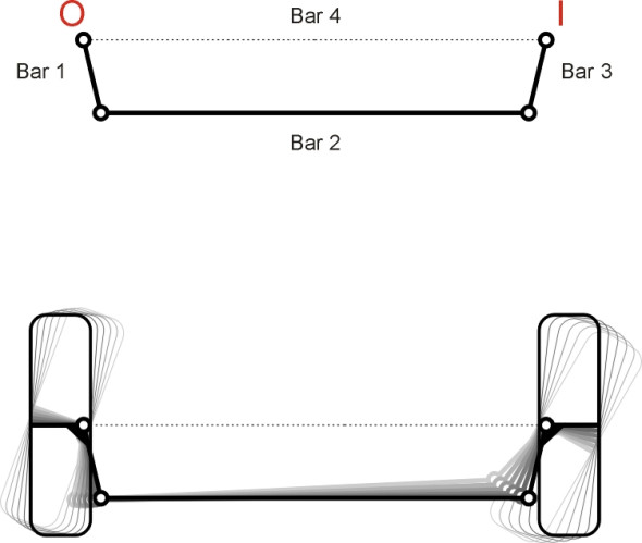
The four-bar linkage

For over 100 years, the geometry of the steering linkage used by most car manufacturers was based on a simple rule of thumb. In this section we shall try to work it using a rigorous mathematical criterion. The aim is to minimise tyre scrub, so the front wheels roll freely and smoothly along their intended paths. In practice, this ‘ideal’ arrangement would only be considered for a slow-moving vehicle such as a mobility scooter. At today’s speeds, the tyres of a standard road vehicle do not actually roll in the direction they are pointing, and the ‘slip angle’ adds a further dimension that takes the problem beyond our scope. Nevertheless, the analysis throws light on the evolution of engineering practice during the early days of the motor car.

Parameters and notation

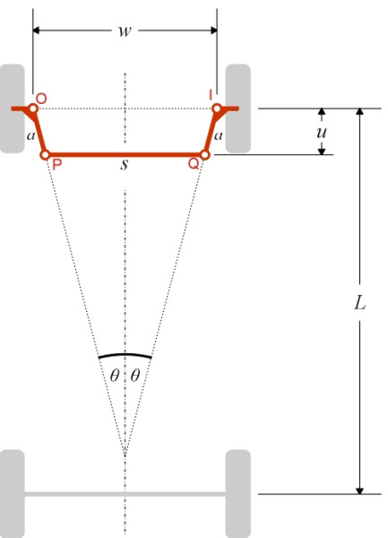
To make a start, we need to attach symbols to the various lengths and angles that define the movement of the linkage. First let’s look at the fixed parameters – the ones that are built into the chassis of the car and don’t change when the wheels are swivelled. There are six of them: $L$, $w$, $a$, $\theta$, $u$, and $s$, as shown in figure 2. $L$ is the distance between the front and rear axles, usually known as the wheelbase. The points O and I are the points where the pivot axes intersect the road surface, and we shall refer to the distance between them as the track width $w$ (this is a simplification - previously we defined the track width as the distance between the wheel centrelines, and although this is not quite the same thing, each pivot axis usually intersects the road very close to the centre of its corresponding contact patch, and it is convenient to assume they coincide). Attached to the wheel hubs are lever arms OP and IQ, each of length $a$. When the steering is in the dead-ahead position, each lever arm makes an angle $\theta$ with the car’s longitudinal axis, and the track rod is spaced a distance $u$ rearward of the front axle centreline. Finally, the two lever arms are linked by the track rod PQ, whose length is denoted by $s$.

Figure 2

For any given model of car, there is not much freedom to change the wheelbase or the track width once the design process has begun. The position of the track rod almost comes into the same category because its position is constrained by the space available behind the engine. Therefore we’ll take $L$, $u$ and $w$ as given. Only one of the remaining three parameters can be varied at will – whichever one we choose, as soon as we fix its value the shape of the mechanism is fully determined. We’ll take $\theta$ as the ‘optional’ parameter. That leaves $a$ and $s$, whose values can be calculated from the others thus:

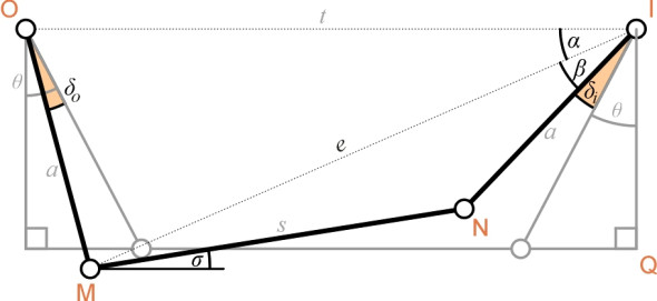
Now for the variables. We assume that the left-hand front wheel swivels to the right through an angle $\delta_o$ (the subscript $o$ indicates that this wheel is the ‘outer’ wheel, i.e., furthest away from the centre of the curve). As it does so, the track rod shifts to the left and rotates anti-clockwise through an angle $\sigma$. In turn, this causes the ‘inner’ wheel to swivel to the right through an angle $\delta_i$ as shown in figure 3. Other quantities whose values change with $\delta_o$ include the angles $\alpha$ and $\beta$ together with the length of the diagonal $e$. They are all functions of $\delta_o$ and strictly speaking they should be written thus: $\sigma ( \delta_o )$, $\delta_i (\delta_o)$, $\alpha (\delta_o)$, and so on. However, we shall omit the arguments for simplicity. We shall also need to differentiate some of these variables with respect to $\delta_o$. We shall use a prime symbol in each case to denote differentiation so that, for example,

Figure 3

The problem

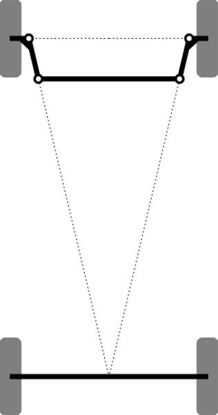
As explained earlier (Section C0505), for many decades it was the custom to arrange the steering arms so that their projections intersect at the rear axle (figure 4). Why? The intention was to minimise tyre scrub, in other words, to make each front wheel roll in the direction it is pointing without any sideways scrubbing of the contact patch. The layout shown in figure 4 became common practice - a rule of thumb that was easy to remember and easy to set up on the drawing board. But it was only an approximation, because for any given set of values of $L$, $w$, $u$ and $\theta$, it turns out that the 4-bar linkage is capable of producing ‘pure’ rolling only at isolated steering positions. We cannot have zero scrub across the whole range. In what follows we will try to work out the arrangement that comes closest to what was intended.

Figure 4

When does the traditional configuration work?

In fact, with the exception of the dead-ahead position, there may be no steering angles at all that produce pure rolling. We can demonstrate this for a car with wheel base 5.0 m, track width 2.5 m, and u = 250 mm. The traditional layout demands that the projections of the two lever arms intersect at the rear axle, so we have

from which we see that $\theta$ is about 16.7$^\circ$.

Let’s make the outer steering angle $\delta_o$ vary step-by step over its full range, and plot the inner steering angle $\delta_i$ that would be required for zero scrub (the formula used to generate this curve is derived in Appendix 1, equation 27). The result is shown in figure 5. This represents the ideal case. The dashed line slopes up to the right at roughly 45$^\circ$, showing the inner wheel must turn more-or-less in unison with the outer wheel. But on closer inspection we see that the slope is not constant: the inner wheel must turn through progressively larger increments relative to the outer wheel as the driver turns the handwheel to the right. This is what one would expect.

Figure 5

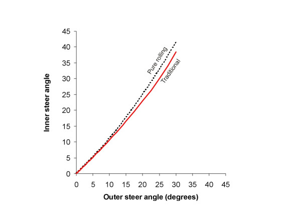
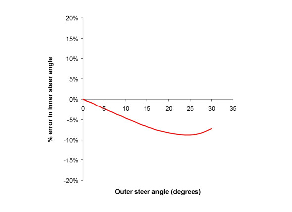
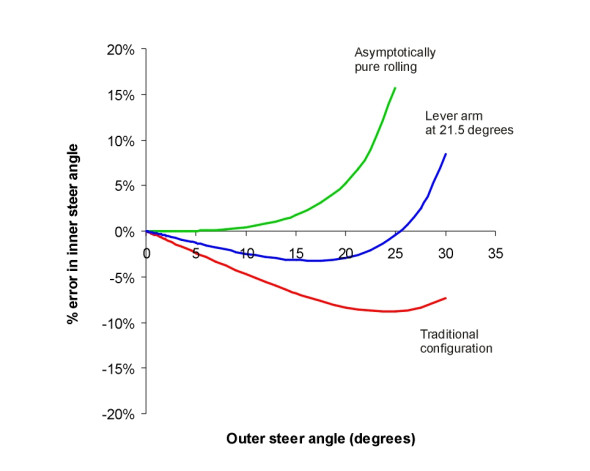
Superimposed on the graph is the actual curve for the 4-bar steering mechanism set at 16.7$^\circ$, represented by the red line (the formula is derived in Appendix 2, equation 35 to equation 38). The two curves don’t seem very different, but if we plot the percentage error in $\delta_i$, that is to say, the percentage difference between the angle needed for pure rolling and what the traditional 4-bar set-up actually produces, we see that it succeeds only when the steering is in the dead ahead position ($\delta_{o}$ = $\delta_{i}$ = 0). Otherwise it falls short across the whole range (figure 6). The inner wheel is not swivelling far enough, and the shortfall rises almost to 10% near full lock. This conclusion remains substantially unchanged even if we increase or decrease the distance $u$ by an appreciable amount.

Figure 6

An ‘improved’ set-up

You may have guessed already that the point of intersection is too far back. In order to persuade the inner wheel to swivel further we need to increase the angle $\theta$. Let’s try 21.5$^\circ$. The result is shown by the blue line in figure 7. The error is now much reduced across most of the range, and we also see that for two particular values of $\delta_o$, namely zero and 25$^\circ$, the correspondence is exact.

Figure 7

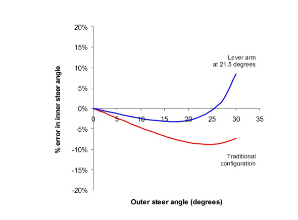
However, we are looking for a set-up such that the error is close to zero for a wider range of values of $\delta_o$, in other words the curve lies close to the x-axis in figure 7 not just in two places but over a considerable range. We want the error to be small especially for low steering angles because drivers spend most of the time with the handwheel close to the dead ahead position when driving at motorway speeds. We might want, in other words, the actual curve to converge asymptotically on the ideal curve as the steering angle $\delta_o$ approaches zero. Clearly, we must increase the angle $\theta$ a bit more yet, but to what value?

Asymptotically pure rolling

Figure 8

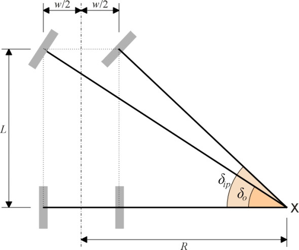
One way to get asymptotically pure rolling is to compare the two equations for the inner steering angle (pure rolling and actual) and see if we can adjust the parameters so that the two equations give the same answer. We’ll distinguish the pure rolling inner steering angle by using the notation $\delta_{ip}$. The geometrical condition for pure rolling is shown in figure 8: the axes of the two front wheels must intersect at the same point X along the axis of the rear axle. The geometry is expressed mathematically via equation 25 to equation 27 in Appendix 1. By rearranging equation 27 we see that the equation for the inner steer angle in pure rolling is

The actual relationship for the 4-bar link is derived in Appendix 2, equation 35 to equation 38, which in a slightly modified form can be written:

where

and

We now know the value of the inner steering angle required for the pure rolling condition, equation 6, and also the inner steering angle for the actual linkage, equation 7. They don’t look at all similar. But we can put them into a similar form by converting each into a power series expansion that is asymptotically true for small $\delta_{o}$. The Maclaurin expansion for $\delta_{ip}$ is

The Maclaurin expansion for $\delta_i$ is

It only remains to work out values for the coefficients. Let’s start with the pure rolling configuration (equation 11). We know that in the central steering position, both steering angles are zero, so $\delta_{ip}$ (0) = 0. The values of $\delta_{ip}'(0)$ and $\delta_{ip}''(0)$ are derived in Appendix 1, equation 32 and equation 34. They are:

Substituting the results in equation 11 gives

Now for the four-bar linkage. In equation 12, we can immediately put $\delta_{i}(0)$ = 0. The values of $\delta_{i}'(0)$ and $\delta_{i}''(0)$ are derived in Appendix 2, equation 45 and equation 46. They are:

Substituting the results into equation 12 gives

Comparing equation 15 and equation 18, we can now see that the four-bar linkage will give asymptotically pure rolling for small steering angles when

or

figure 9 shows the resulting geometry: for asymptotically pure rolling, the point of intersection of the steering arms should be located a distance $\frac{1}{2} L + u$ behind the front axle. This is very different from the traditional configuration, and we’ll consider the implications later. Finally, we plot the error curve for this steering geometry applied to the car that we looked at earlier. The result is indicated by the green curve in figure 10, which indicates that the error is extremely small for all steering angles up to about 10 degrees. The snag is that the error rises quite quickly thereafter, showing that the inner wheel swivels too far as the outer wheel approaches full lock. We’ll say more about this configuration this later.

Figure 9

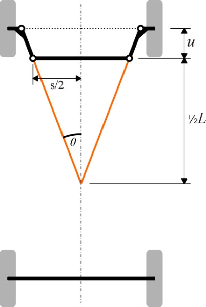
Figure 10

The rack-and-pinion linkage

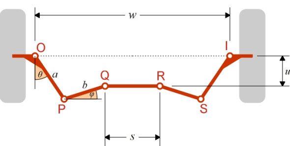
The four-bar linkage was standard throughout the first hundred years of automobile construction, but has now been superseded by rack-and-pinion steering in which the rack slides from side-to-side in a guideway (figure 11). The fixed geometrical parameters are shown in figure 12. They include as before the wheelbase $L$, track width $w$, track rod set-back $u$, steering lever arm length $a$, and steering arm angle $\theta$. The length $b$ of the steering links PQ and RS, the length $s$ of the centre section, and the steering link angle $\phi$ are new. Note that of all the eight parameters listed, $a$ and $b$ are redundant, since the geometry is completely defined by the other six. Also, the angle $\phi$ can be negative, and so can the setback $u$, and each of these possibilities leads to a variation that may appear geometrically distinct but in fact obeys the same mathematical equations.

Figure 11

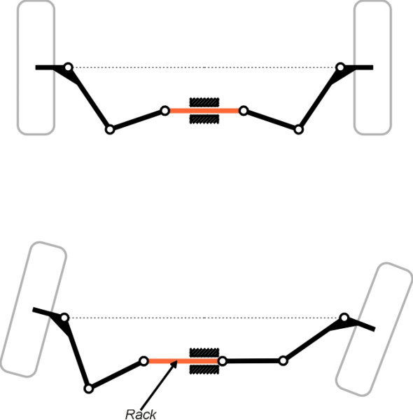
Figure 12

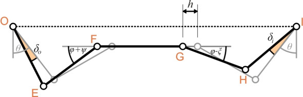
The variables are the outer and inner steering angles $\delta_{o}$ and $\delta_{i}$, the angles of rotation $\psi$ and $\xi$ (both positive anticlockwise) of the two steering links, and the lateral motion $h$ of the rack. All are shown in figure 13. As in the previous analysis, we treat each of the variables $\delta_{i}$, $\psi$, $\xi$, and $h$ as functions of $\delta_{o}$.

Figure 13

In principle, this configuration can be analysed in the same way as the traditional four-bar linkage, although the geometry is more complicated and the author has not been able to derive a formula for the inner steering angle $\delta_{i}$ explicitly in terms of the outer steering angle $\delta_{o}$. Again we can express the inner steering angle as a power series expansion of the outer steering angle and compare the coefficients with those required for pure rolling. The values of the coefficients $\delta_{i}'(0)$ and $\delta_{i}''(0)$ are derived in Appendix 3, equation 65 and equation 66. They are:

If we substitute these expressions into the Maclaurin expansion equation 12 we get:

Finally, comparing the coefficient of $\delta_{o}^{2}$ with the corresponding coefficient in equation 15 leads to the condition we seek for asymptotically pure rolling at small steering angles, thus:

To summarise, provided the angles $\theta$ and $\phi$ together with the dimensions $a$, $b$, $w$ and $L$ satisfy equation 24, the front wheels will be in the correct alignment for zero scrub at small steering angles.

Conclusion

If the purpose of the Ackermann steering linkage is to minimise scrub at small steering angles, the theoretically optimum layout requires the point of intersection of the lever arms to be located close to the centre of the vehicle wheelbase. This is further forward than the traditional layout for early cars, and as the technology progressed some manufacturers did indeed move the intersection point forward to a location roughly two thirds of the wheelbase from the front axle [2]. Since then, the situation has changed completely, because the modern trend is to go the other way [1]. With the four-bar linkage, this means fixing the point of intersection of the steering arms aft of the rear axle. This has the advantage that the inside wheel then swivels through a smaller angle at full lock, which in turn reduces size of the wheel housing where it intrudes into the passenger cabin. But a more important reason is that the car handles better. At high speeds, the assumptions underlying the ‘pure rolling’ analysis no longer apply, because the wheels don’t move in the direction they are pointing. The tyre slip angles (see Section C1717) become significant, and since load is transferred from the inside to the outside wheel on any curve, the inside and outside slip angles will be different. In order to maximise grip, suspension designers aim for a higher slip angle on the outside tyre, which means a reduced degree of Ackermann compensation.

But within a few years, all these considerations could swept aside. It will soon be possible to build cars with a computer-controlled steering system in which the front wheels swivel independently, driven by electrically-powered actuators. An electrical signal from the driver’s handwheel will be interpreted by a microprocessor that modifies the steering angles to take into account the speed of the car, the radius of turn, and the wheel loads at the time. Since there will be no steering column and no track rod, the handwheel unit can be bolted to any suitable surface inside the passenger cabin. In this sense the driver will lose all direct contact with the road outside, and cues that previously arrived through the handwheel will be replaced through artificially-induced feedback. Instead, the computer will take over some of the responsibility and set up the steering angles to get the best out of the tyres and the road surface. The car will become more intelligent and sure-footed, a little bit like a horse.